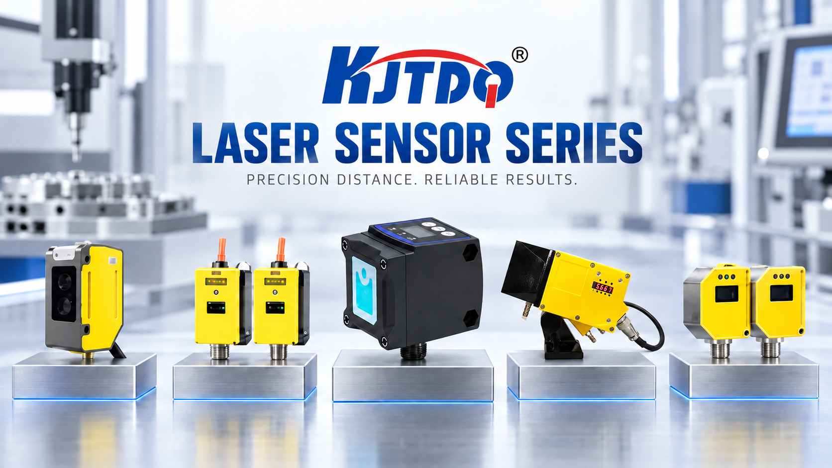
The choice between laser triangulation and time-of-flight measurement is decided by the tolerance on the drawing, not by the technology: triangulation delivers micrometre-level repeatability over distances measured in tens of millimetres, while time-of-flight covers metres at millimetre-level accuracy. Matching one of those two bands to the tolerance the drawing already specifies is the whole specification exercise. KJT Sensors manufactures both classes — miniature CMOS triangulation sensors with repeatability from 10 μm across standard sensing distances of 30 mm to 400 mm, and laser distance sensors with measuring ranges from 0.05 m to 10 m, including amplifier-built-in time-of-flight models — so an application can be examined at either end of the accuracy–range trade-off before hardware is selected.
What a Displacement Sensor Measures That a Distance Sensor Does Not
A displacement sensor reports change against a reference. A distance sensor reports absolute distance from the sensor face. The distinction sounds academic until the inspection drawing arrives: thickness, step height, flatness, and warpage are all differences, and a difference can be measured far more precisely than an absolute distance.
Three properties follow from measuring change over a short working range.
- Resolution improves as the working range shrinks. A device that only has to resolve a few millimetres of travel can spend its entire optical budget on precision, which is why micrometre repeatability is available at short range and not at long range.
- The reference can be taught on site. Datum mode, one-point, two-point, and three-point teaching let the sensor treat a known surface as zero, so a fixture that is imprecise but repeatable still produces accurate inspection results.
- A single value drives both a measurement and a decision. The KJT triangulation family outputs a real-time distance value and a switching signal simultaneously, which allows one sensor to feed a process trend to the controller and an OK/NG judgment to the line at the same time.
Triangulation: How Geometry Buys Micrometres at Short Range
In a triangulation sensor, a laser is projected onto the target at an angle and the reflected spot is imaged onto a CMOS receiving element. Movement of the target shifts the position of the spot on the receiver, and the shift is converted into distance by trigonometry. Because the geometry is amplified across the receiver rather than measured in time, very small displacements produce measurable spot movement.
The KJT miniature CMOS triangulation range is structured as a ladder of five accuracy classes, and reading the ladder explains both the technology and its limits.
- 30 mm sensing distance, ±5 mm measuring range — repeatability 10 μm, linearity error ±0.1% F.S., beam diameter φ50 μm.
- 50 mm sensing distance, ±15 mm measuring range — repeatability 30 μm, linearity ±0.1% F.S., beam φ70 μm.
- 100 mm sensing distance, ±35 mm measuring range — repeatability 70 μm, linearity ±0.1% F.S., beam φ120 μm.
- 200 mm sensing distance, ±80 mm measuring range — repeatability 200 μm, linearity ±0.2% F.S., beam φ300 μm.
- 400 mm sensing distance, ±200 mm measuring range — repeatability 300 to 800 μm, linearity ±0.2 to 0.3% F.S., beam φ500 μm.
Two conclusions can be read directly from that ladder of classes. Precision and standoff trade against each other by roughly an order of magnitude across the family, so precision is highest at the shortest sensing distance. The beam diameter grows with the standoff at the same time, which is why the finest features can be resolved at the shortest distances. Both classes emit a 655 nm Class 2 laser, in a die-cast aluminum alloy housing rated IP67, with a temperature characteristic of 0.03% F.S./°C.
Time-of-Flight: Range Without a Reflector, at Millimetre Accuracy
Time-of-flight sensors measure the round-trip travel time of a short light pulse or the phase relationship of a modulated beam. The geometry constraints of triangulation disappear, so the technique works at distances of metres and tolerates targets that triangulation finds difficult.
The KJT laser distance range covers 0.05 m to 10 m at 90% reflectance, with absolute accuracy of ±10 mm referred to maximum range and improved accuracy at shorter distances, repeatability of 3 mm, output frequency of 40 Hz with 1 to 2 kHz available on adjustable models, and a 4 mm spot at 1 m. The published performance is reliable on dark, shiny, and angled surfaces, which is the specification that matters on black rubber, bare aluminum, or wet product.
The two principles therefore divide the work along a clear line.
- Tolerance tighter than about ±0.5 mm — triangulation, mounted close to the target.
- Tolerance around ±10 mm or looser, at distances of metres — time-of-flight.
- Target hot, far away, or moving fast — time-of-flight, with the response time checked against the speed.
- Feature smaller than the beam spot — triangulation at short range, because the spot is measured in tens of micrometres.
Repeatability, Linearity, and Accuracy Are Three Different Numbers
A requirement written as “±1 mm accuracy” sits in a comfortable place for both technologies, and that is exactly why it is worth separating the three numbers that get collapsed into the word accuracy.
- Repeatability describes how closely the sensor returns to the same reading when the target returns to the same position. It is the number that governs OK/NG sorting consistency, and it is the smallest figure on a triangulation datasheet.
- Linearity error describes the maximum deviation from a straight line across the measuring range, expressed as a percentage of full scale. On a ±5 mm range, a ±0.1% F.S. figure corresponds to about 10 μm; on a ±200 mm range, ±0.2% F.S. corresponds to about 800 μm.
- Accuracy is what remains after repeatability, linearity, temperature effects, target effects, and mounting error are combined. The combined figure is worse than either of the first two numbers, and it is the figure a gauge repeatability study will eventually produce.
The temperature characteristic is the number that surprises people. At 0.03% F.S./°C, a sensor on a ±5 mm range drifts by roughly 3 μm per °C, so a 30 °C night-to-afternoon swing in an unheated shop contributes about 90 μm. The same specification applied to a ±200 mm range drifts by roughly 120 μm per °C, which over the same 30 °C swing exceeds 3 mm — more than a ±1 mm tolerance on its own.
The practical rule that follows is to specify the smallest measuring range that still covers the process window. Buying standoff you do not need costs accuracy you cannot recover, and the loss is invisible on the datasheet because it appears only when the temperature moves.
Inline Thickness and Coating Measurement on Thin Materials
Thickness cannot be measured reliably by a single sensor looking at one surface, because both surfaces move. Two arrangements are standard.
- Differential measurement places two sensors on opposite sides of the material and subtracts the two readings. The subtraction cancels common-mode movement, so web flutter and line vibration largely disappear from the result. This is the configuration used for coating thickness on battery electrodes, adhesive layers, films, and thin sheet.
- Reference-roller measurement places a single sensor against a roller of known diameter and measures the gap to the material wrapped over it. One sensor replaces two, at the cost of an assumption about the roller.
Sampling rate then has to be matched to line speed. Response time on the KJT triangulation family is selectable at 1.5 ms, 5 ms, or 10 ms. At the 1.5 ms setting a single sensor produces roughly 600 readings per second, which at a line speed of 1 m/s means one measurement every 1.5 mm of travel; a 5 mm coating defect is therefore sampled about three times. Moving to a faster line or a smaller defect requires either a faster sensor or a narrower inspection window, and the arithmetic is worth doing before the purchase order rather than after.
Step, Height, and Flatness Inspection on Metal Sheet and Workpieces
Geometric inspection uses the same sensor in a different role: the target is stationary or traversing, and the question is where the surface sits relative to a taught reference.
- Step and height measurement compares two surfaces. The measuring range has to span the step, and the repeatability determines the smallest step that can be judged reliably.
- Flatness and warpage are derived from a series of readings along a surface. Peak-hold and valley-hold functions capture the extremes without a high-speed controller, and zero-reset allows the operator to re-reference the fixture between batches.
- Tolerance sorting uses the switching output against taught high and low limits, with light-ON or dark-ON logic to suit the controller. Micro-height differences on stamped parts, connector pins, and laminated cores are typical work.
- Deformation and vibration monitoring on a machine frame uses the sensor as a low-cost displacement transducer rather than as an inspection gauge, with the switching output wired to a condition alarm.
The data quality in all four cases depends on the same two things: the spot is smaller than the feature being judged, and the fixture holds the standoff stable to within the repeatability being claimed.
Surface Defect Detection: Spot Size Against Feature Size
Surface inspection is where the beam diameter decides whether an application is feasible at all.
A φ50 μm spot at 30 mm can resolve pitting, scratches, and edge burrs on a machined surface, and the resulting profile is a genuine metrology result. The same inspection attempted with a φ500 μm spot at 400 mm averages the defect into the surrounding surface and reports a surface that looks flat, because the instrument did not resolve the defect — it measured the average of the defect and its surroundings. Neither sensor is at fault; the spot size and the defect size were not compared before the task was quoted.
Practical limits to check before quoting a surface inspection task:
- Feature size against spot size — the spot should be no larger than the smallest defect that has to be detected.
- Scan speed against response time — a traversing sensor covers the line speed of the axis, so the number of readings per millimetre of surface follows from the response time.
- Surface finish against incidence angle — polished, machined, and rolled surfaces scatter differently, and the mounting angle should be adjusted so that the specular reflection does not run straight back into the receiver.
When a Single Point Is Not Enough: 2D and 3D Inspection
A single-point sensor describes one line on the surface as the axis traverses it. Full-field inspection is a different instrument class.
- A 2D scanning laser sweeps a beam and reports distance across an angular field, which covers an area rather than a line and is used for area guarding, profile scanning, and volume work. KJT manufactures a scanning laser model specified for coverage up to 50 m.
- A line-profile sensor projects a laser line and images it, producing a full cross-section in one exposure, which is the usual route for bead inspection, gap and flush measurement, and continuous profile logging.
- Machine vision applies where the question is appearance rather than geometry: print quality, labels, surface discoloration. KJT supplies visual defect detection systems for automated surface inspection.
- Single-point triangulation remains the right instrument where the tolerance is measured in micrometres and the feature is a point measurement rather than a surface judgment.
Mounting, Interface, and the Details That Decide Uptime
The mechanical and electrical details of the installation decide whether the specified precision reaches the process.
- Body and mounting. A 20 × 44 × 25 mm die-cast aluminum body weighing approximately 35 g can be mounted directly on a machine member through integrated countersunk holes, on an adjustable stainless-steel bracket where the angle has to be trimmed. The bracket families used with these compact sensors are widely standardized, which simplifies retrofits.
- Electrical. Supply is 12 to 24 V DC with ripple limited to 10% peak-to-peak, current consumption is ≤40 mA, output is NPN or PNP open collector with a maximum load current of 50 mA and residual voltage ≤1.5 V, and short-circuit protection is built in with automatic reset.
- Environment. Operating ambient temperature is −10 °C to +55 °C, with storage to +65 °C, and the die-cast housing resists deformation and temperature drift.
- Commissioning. One-touch teaching in one, two, or three points, zero reset, power-on and operation delays, a fixed 5 ms one-shot output, and a parameter key lock cover the setup work that otherwise consumes a commissioning shift.
- Diagnostics. Self-check, contamination warning, and service-life warning are available, and measured values, status, received light level, and fault codes can be uploaded over IO-Link together with automatic parameter download.
Cross-Referencing an Existing Triangulation Sensor
Where a compact triangulation sensor is already installed inside a machine, the replacement decision is usually driven by dimensional and electrical compatibility rather than by datasheet performance. The KJT miniature CMOS family is published as dimensionally and functionally compatible with the widely used compact triangulation sensors in the corresponding sensing-distance classes, down to matching sensing distances, measuring ranges, repeatability classes, and beam diameters, and is available in standard bodies with a 2 m fixed cable or in M12 connector versions.
A replacement checklist keeps the exercise honest:
- Sensing distance and measuring range — both, not one, and with the process window inside the range rather than at its edge.
- Repeatability class — replacing a precision class with a coarse one will pass the wiring check and fail the inspection.
- Output and interface — NPN or PNP open collector, plus IO-Link where parameters are managed from a controller.
- Cable or connector, and body envelope — a fixed cable cannot be swapped for an M12 connector without rework of the cable run.
- Teaching method — one, two, or three-point teaching has to match how the maintenance team is used to setting the device.
Where KJT Sensors Fits
KJT Sensors is the international brand of Nanjing KJT Electric Co., Ltd., an industrial sensor manufacturer established in 2010. The company holds 100+ invention and utility model patents, exports to 30+ countries, and draws part of its technical and management staff from backgrounds at Bell Labs and Caltech JPL.
Compliance coverage includes ISO 9001, ISO 14001, and ISO 45001 management system certification, product certification to CE, RoHS, CCC, and SIL, and enclosure protection spanning IP65, IP67, IP68, and IP69K across the product range.
The laser portfolio covers distance measurement, high-precision distance measurement, high-frequency measurement, displacement, liquid level, hot and cold metal detection, ranging modules, and explosion-proof distance measurement, with a scanning laser covering area work. A food group uses KJT laser sensors for packaging box dimension inspection and stack height measurement, where the visible laser spot shortened alignment and non-contact measurement kept the product uncontaminated — the same combination of geometric judgment and non-contact measurement that precision manufacturing lines need.
https://www.kjt-sensors.com/
KJT Sensors